3. California Regional Model

3.1. Overview

This regional model is constructed in the eastern Pacific Ocean and encompasses most of the California current region. This model is constructed to run during the year 2008 and is initiated and forced with output from the ECCO Version 5 Alpha State Estimate. The domain of the regional model is shown in the following plot:

3.1.1. eccoseas modules

The construction of this model showcases many of the components of the eccoseas package in the downscale and ecco modules. These modules are used in this demo to complete the following list of tasks:

1. Bathymetry “filling” to remove isolated regions

2. Reading the ECCO grid

3. Reading ECCO Version 5 output fields

4. Reading ECCO external forcing fields

5. Interpolating 2D and 3D fields to a regional domain for initial, external, and boundary conditions

3.1.2. Required ECCO Data

For this example, the following list of files are required from the ECCO Version 5 Alpha State estimate. These files are available on the ECCO drive.

ECCO files required to construct the California regional model

Variable	File(s)
Potential Temperature	THETA_2007.nc, THETA_2008.nc, THETA_2009.nc
Salinity	SALT_2007.nc, SALT_2008.nc, SALT_2009.nc
u-Component of Velocity	UVELMASS_2007.nc, UVELMASS_2008.nc, UVELMASS_2009.nc
v-Component of Velocity	VVELMASS_2007.nc, VVELMASS_2008.nc, VVELMASS_2009.nc
Sea Surface Height Anomaly	ETAN_2007.nc, ETAN_2008.nc, ETAN_2009.nc
Lowngwave Downwelling Radiation	EIG_dlw_plus_ECCO_v4r1_ctrl_2008
Shortwave Downwelling Radiation	EIG_dsw_plus_ECCO_v4r1_ctrl_2008
u-Component of Wind	EIG_u10m_2008
v-Component of Wind	EIG_v10m_2008
Precipitation	EIG_rain_plus_ECCO_v4r1_ctrl_2008
Air Temperature	EIG_tmp2m_degC_plus_ECCO_v4r1_ctrl_2008
Specific Humidity	EIG_spfh2m_plus_ECCO_v4r1_ctrl_2008
Grid components for each tile	GRID.0001.nc through GRID.0013.nc

3.1.3. Configuration Files

The model configuration files for this regional model are provided in the configurations directory of the eccoseas Github repository.

The following sections showcase the construction of the input binaries for the model.

3.2. Model Grid

• 3.2.1. Constructing the Grid
  • 3.2.1.1. Visualizing the Grid
  • 3.2.1.2. Visualizing the Grid on a Map with Cartopy
  • 3.2.1.3. Visualizing the Grid Spacing

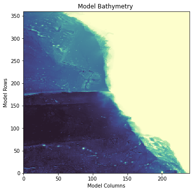
3.3. Bathymetry

• 3.3.1. Generating the Bathymetry Grid
  • 3.3.1.1. Interpolating Bathymetry onto the Model Domain
  • 3.3.1.2. Visualizing the Bathymetry Grid
  • 3.3.1.3. Checking for isolated regions
  • 3.3.1.4. Manually checking for problem areas

3.4. Initial Conditions

• 3.4.1. Constructing the Initial Conditions
  • 3.4.1.1. Step 1: Download the ECCO fields
  • 3.4.1.2. Step 2: Read in the ECCO grid
  • 3.4.1.3. Step 3: Read in the Model Grid and Generate a Mask
  • 3.4.1.4. Step 4: Prepare the grids for interpolation
  • 3.4.1.5. Step 5: Interpolate the Fields onto the Model Grid
  • 3.4.1.6. Step 6: Plotting the Initial Condition Fields
  • 3.4.1.7. Step 7: Run-time considerations

3.5. External Forcing Conditions

• 3.5.1. Constructing External Forcing Files
  • 3.5.1.1. Step 1: Download the ECCO external forcing fields
  • 3.5.1.2. Step 2: Read in the external forcing fields
  • 3.5.1.3. Step 3: Read in the Regional Model Grid
  • 3.5.1.4. Step 4: Interpolate the Fields onto the Model Grid
  • 3.5.1.5. Step 5: Plotting the External Forcing Fields

3.6. Boundary Conditions

• 3.6.1. Constructing the Boundary Conditions
  • 3.6.1.1. Step 1: Download the ECCO fields
  • 3.6.1.2. Step 2: Read in the ECCO grid
  • 3.6.1.3. Step 3: Read in the Model Grid and Generate a Mask
  • 3.6.1.4. Step 4: Prepare the grids for interpolation
  • 3.6.1.5. Step 5: Interpolate the Fields onto the Model Grid
  • 3.6.1.6. Step 6: Plotting the Boundary Fields