Up next, we will generate the external forcing conditions that will be used in the California regional model.

First, import packages create and visualize the model fields here:

# import the modules for computation, plotting, and reading files
import os
import numpy as np
from scipy.interpolate import griddata
import matplotlib.pyplot as plt
from scipy.interpolate import griddata
from matplotlib.gridspec import GridSpec
import netCDF4 as nc4
import cmocean.cm as cm

# import the necessary modules from eccoseas
from eccoseas.ecco import exf
from eccoseas.ecco import io
from eccoseas.downscale import hFac
from eccoseas.downscale import horizontal

3.5.1. Constructing External Forcing Files

For this example, we will use the external forcing fields from the ECCO Version 5 state estimate. We will prepare these fields in 5 steps:

1. download 7 external forcing fields used in the ECCO model

2. read the external forcing fields used in the ECCO model as well as the ECCO grid

3. read in the bathymetry for the regional model as well as its grid

4. interpolate the ECCO fields onto the regional model grid and store each as a binary file

5. plot the interpolated fields to ensure they look as expected

3.5.1.1. Step 1: Download the ECCO external forcing fields

To begin, download the ECCO external forcing fields used in the ECCO Version 5 Alpha state estimate. These fields are available HERE. For this regional model, we will downloaded the following list of files forfor the year 2008:

Variable	File Name
ATEMP	EIG_tmp2m_degC_plus_ECCO_v4r1_ctrl
AQH	EIG_spfh2m_plus_ECCO_v4r1_ctrl
SWDOWN	EIG_dsw_plus_ECCO_v4r1_ctrl
LWDOWN	EIG_dlw_plus_ECCO_v4r1_ctrl
UWIND	EIG_u10m
VWIND	EIG_v10m
PRECIP	EIG_rain_plus_ECCO_v4r1_ctrl

These fields are stored in the following direectory:

data_folder = '../../../data/california'

3.5.1.2. Step 2: Read in the external forcing fields

To read in the ECCO fields, I will rely on the exf module from the eccoseas package. We will loop through all of the files we downloaded, reading them in with the exf module:

# make a file dictionary to loop over
file_prefix_dict = {'ATEMP':'EIG_tmp2m_degC_plus_ECCO_v4r1_ctrl',
                    'AQH':'EIG_spfh2m_plus_ECCO_v4r1_ctrl',
                    'SWDOWN':'EIG_dsw_plus_ECCO_v4r1_ctrl',
                    'LWDOWN':'EIG_dlw_plus_ECCO_v4r1_ctrl',
                    'UWIND':'EIG_u10m',
                    'VWIND':'EIG_v10m',
                    'PRECIP':'EIG_rain_plus_ECCO_v4r1_ctrl'}

variable_names = list(file_prefix_dict.keys())

# make a list to hold all of the exf grids
exf_grids = []
year=2008

# loop through each variable to read in the grid
for field in variable_names:
    exf_lon, exf_lat, exf_grid = exf.read_ecco_exf_file(data_folder, file_prefix_dict[field], year)
    exf_grids.append(exf_grid)

With an eye toward the interpolation that will come in step 4, we will make 2D grids of longitudes and latitudes to use in the interpolation

Exf_Lon, Exf_Lat = np.meshgrid(exf_lon, exf_lat)
ecco_points = np.column_stack([Exf_Lon.ravel(), Exf_Lat.ravel()])

We can visualize these grids as follows:

ecco_meta_dict = {'ATEMP':[-50, 30, cm.thermal, '$^{\circ}$C'],
             'AQH':[0, 0.025, cm.tempo, 'kg/kg'],
             'PRECIP':[0, 1e-6, cm.tempo, 'm/s'],
             'SWDOWN':[-1000,0,cm.solar,'W/m$^2$'],
             'LWDOWN':[-500, 0,cm.solar,'W/m$^2$'],
             'UWIND':[-20, 20, cm.balance, 'm/s'],
             'VWIND':[-20, 20, cm.balance, 'm/s']}
ecco_variable_names = list(ecco_meta_dict.keys())

fig = plt.figure(figsize=(8,10))
gs = GridSpec(4, 2, wspace=0.4, hspace=0.03,
              left=0.11, right=0.9, top=0.95, bottom=0.05)


for i, exf_grid in enumerate(exf_grids):
    variable_name = ecco_variable_names[i]

    # choose just the first timestep for plotting
    exf_grid = exf_grid[0, :, :]

    ax1 = fig.add_subplot(gs[i])
    C = plt.pcolormesh(Exf_Lon, Exf_Lat, exf_grid,
                       vmin=ecco_meta_dict[variable_names[i]][0],
                       vmax=ecco_meta_dict[variable_names[i]][1],
                       cmap=ecco_meta_dict[variable_names[i]][2])
    plt.colorbar(C, label=variable_names[i]+' ('+ecco_meta_dict[variable_names[i]][3]+')',fraction=0.026)

    if i<5:
        plt.gca().set_xticklabels([])
    else:
        plt.gca().set_xlabel('Longitude')
    if i%2==1:
        plt.gca().set_yticklabels([])
    if i==7:
        plt.gca().axis('off')
    if i==2:
        plt.gca().set_ylabel('Latitude')

plt.show()

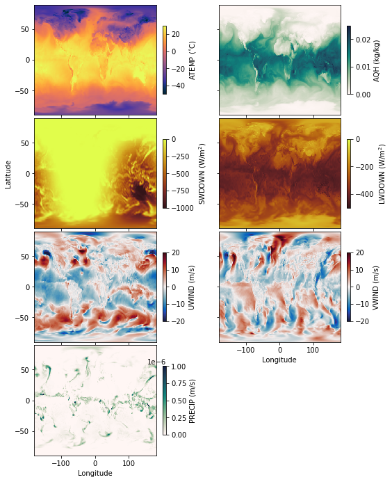
As we can see, the external forcing fields are global - and we can use this to our advantage in the interpolation since we don’t need to “spread” these variable like the oceanic variables.

3.5.1.3. Step 3: Read in the Regional Model Grid

Next, we will recreate the grid we will use in the regional model and read in the bathymetry file (see previous notebooks for details) in order to generate the land mask:

# define the input directory (constructed in the previous notebook for bathymetry)
# this directory should already have the bathymetry file called CA_bathymetry.bin
input_dir = '../../../configurations/california/input'

# define the parameters that will be used in the data file
delX = 1/12
delY = 1/16
xgOrigin = -135
ygOrigin = 29
n_rows = 360
n_cols = 240

# recreate the grids that will be used in the model
xc = np.arange(xgOrigin+delX/2, xgOrigin+n_cols*delX, delX)
yc = np.arange(ygOrigin+delY/2, ygOrigin+n_rows*delY+delY/2, delY)
XC, YC = np.meshgrid(xc, yc)

# read in the bathymetry file
bathy = np.fromfile(os.path.join(input_dir,'CA_bathymetry.bin'),'>f4').reshape(np.shape(XC))

# create the surface mask
ecco_DRF_tiles = io.read_ecco_grid_tiles_from_nc(data_folder, var_name='DRF')
delR = ecco_DRF_tiles[1]
surface_mask = hFac.create_hFacC_grid(bathy, delR)[0,:,:]
surface_mask[surface_mask>0]=1
surface_mask = surface_mask.astype(int)

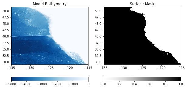
To double check the mask was created as expected, we will plot it in comparison to the bathymetry here:

plt.figure(figsize=(10,5))

plt.subplot(1,2,1)
C = plt.pcolormesh(XC, YC, bathy, vmin=-5000, vmax=0, cmap='Blues_r')
plt.colorbar(C, orientation = 'horizontal')
plt.title('Model Bathymetry')

plt.subplot(1,2,2)
C = plt.pcolormesh(XC, YC, surface_mask, vmin=0, vmax=1, cmap='Greys')
plt.colorbar(C, orientation = 'horizontal')
plt.title('Surface Mask')

plt.show()

3.5.1.4. Step 4: Interpolate the Fields onto the Model Grid

Next, we will interpolate the ECCO external fields Iwe read in onto the regional model domain. Since spreading is not necessary, we can just use the scipy package for interpolation. This interpolation is bundled efficiently into the downscale_exf_field function in eccoseas.

# ensure the output folder exists
if 'exf' not in os.listdir(input_dir):
    os.mkdir(os.path.join(input_dir, 'exf'))

# tri is the interpolation model and only needs to be computed once
# it is reused after it is computed in the downscale function
tri = None

# loop through each variable and corresponding ECCO grid
for variable_name, exf_grid in zip(variable_names, exf_grids):

    # print a message to keep track of which variable we are working on
    print('    - Interpolating the '+variable_name+' grid')

    # create a grid of zeros to fill in
    interpolated_grid, tri = horizontal.downscale_exf_field(ecco_points, exf_grid,
                                                          XC, YC, surface_mask, tri)

    # convert ECCO values to MITgcm defaults
    if variable_name=='ATEMP':
        interpolated_grid += 273.15
    if variable_name in ['SWDOWN','LWDOWN']:
        interpolated_grid *=-1

    # output the interpolated grid
    output_file = os.path.join(input_dir,'exf',variable_name+'_'+str(year))
    interpolated_grid.ravel('C').astype('>f4').tofile(output_file)

    - Interpolating the ATEMP grid
    - Interpolating the AQH grid
    - Interpolating the SWDOWN grid
    - Interpolating the LWDOWN grid
    - Interpolating the UWIND grid
    - Interpolating the VWIND grid
    - Interpolating the PRECIP grid

3.5.1.5. Step 5: Plotting the External Forcing Fields

Now that the fields have been generated, we will plot them to ensure they look as expected. First, generate some metadata for each one:

meta_dict = {'ATEMP':[273, 290, cm.thermal, '$^{\circ}$C'],
             'AQH':[0, 0.025, cm.tempo, 'kg/kg'],
             'PRECIP':[0, 1e-6, cm.tempo, 'm/s'],
             'SWDOWN':[-10,20,cm.solar,'W/m$^2$'],
             'LWDOWN':[-100, 500,cm.solar,'W/m$^2$'],
             'UWIND':[-20, 20, cm.balance, 'm/s'],
             'VWIND':[-20, 20, cm.balance, 'm/s'],
             'RUNOFF':[0, 2e-8, cm.tempo, 'm/s']}

Then, create all of the subplots:

fig = plt.figure(figsize=(8,10))
gs = GridSpec(4, 2, wspace=0.4, hspace=0.03,
              left=0.11, right=0.9, top=0.95, bottom=0.05)


for i in range(len(variable_names)):
    variable_name = variable_names[i]

    CA_exf_grid = np.fromfile(os.path.join(input_dir,'exf',variable_name+'_'+str(year)),'>f4')
    CA_exf_grid = CA_exf_grid.reshape((np.shape(exf_grid)[0],np.shape(XC)[0], np.shape(XC)[1]))

    # choose just the first timestep for plotting
    CA_exf_grid = CA_exf_grid[0, :, :]

    ax1 = fig.add_subplot(gs[i])
    C = plt.pcolormesh(XC, YC, CA_exf_grid,
                       vmin=meta_dict[variable_names[i]][0],
                       vmax=meta_dict[variable_names[i]][1],
                       cmap=meta_dict[variable_names[i]][2])
    plt.colorbar(C, label=variable_names[i]+' ('+meta_dict[variable_names[i]][3]+')',fraction=0.026)

    if i<5:
        plt.gca().set_xticklabels([])
    else:
        plt.gca().set_xlabel('Longitude')
    if i%2==1:
        plt.gca().set_yticklabels([])
    if i==7:
        plt.gca().axis('off')
    if i==2:
        plt.gca().set_ylabel('Latitude')

plt.show()

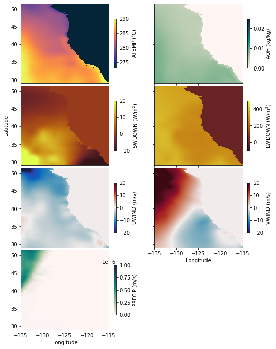
Looks good! Next, we’ll take a look at the boundary conditions.