5. Alaska Slope Regional Model

5.1. Overview

This is a description of the AK model

The construction of this model showcases many of the components of the eccoseas package in the downscale and ecco modules.

This model example will showcase the following updates not previously shown in the previous model examples:

1. Constructing pickup files for regional models given pickups from global models

2. Working with passive tracers (used for biogeochemical packages)

The functions used in this demo include the tasks in the following list:

1. Reading and writing pickup files

2. Interpolating 2D and 3D grids to regional domains

5.1.1. Required ECCO Data

The initial conditions for this model will be generating using existing pickup files from the ECCO-Darwin solution. The list of pertainent files is listed here:

ECCO-Darwin files required to construct the Alaska North Slope regional model

Description	File(s)
Physical Variables Pickup	pickup.0000000001.data, pickup.0000000001.meta
Seaice Variables Pickup	pickup_seaice.0000000001.data, pickup_seaice.0000000001.meta
Darwin Variable Pickup (pH)	pickup_darwin.0000000001.data, pickup_darwin.0000000001.meta
Darwin Tracers Pickup	pickup_ptracers.0000000001.data, pickup_ptracers.0000000001.meta

In addition to the data above, we also need the grid information. We read this in from the nctiles_grid section of the ECCO Drive:

ECCO grid files required to construct the Alaska North Slope regional model

Description	File(s)
Grid description	tile001.mitgrid, tile002.mitgrid, tile003.mitgrid, tile004.mitgrid, tile005.mitgrid
Grid angles	AngleCS.data, - AngleSN.data
Grid wet masks	hFacC.data, hFacS.data, hFacW.data

5.2. Model Grid

• 5.2.1. Reading the grid
  • 5.2.1.1. Visualizing the Grid
  • 5.2.1.2. Visualizing the Grid on a Map with Cartopy
  • 5.2.1.3. Visualizing the Grid Spacing

5.3. Interpolation Grid

• 5.3.1. Motivation for an Interpolation Grid
• 5.3.2. Constructing the Interpolation Grid
  • 5.3.2.1. Step 1: Download the ECCO Files
  • 5.3.2.2. Step 2: Read in the ECCO grid
  • 5.3.2.3. Step 3: Read in the Regional Model Grid and Mask
  • 5.3.2.4. Step 4: Prepare the grids for interpolation
  • 5.3.2.5. Step 5: Interpolate the ECCO mask vertically
  • 5.3.2.6. Step 6: Reprojecting the Model Grid
  • 5.3.2.7. Step 7: Creating the Interpolation Grid
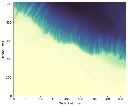
  • 5.3.2.8. Step 8: Visualizing the Interpolation Grid

5.4. Initial Conditions

• 5.4.1. Constructing the Initial Conditions
  • 5.4.1.1. Step 1: Download the ECCO Files
  • 5.4.1.2. Step 2: Read in the Regional Model Grid and Mask
  • 5.4.1.3. Step 3: Read in the pickup file and the ECCO grid
    • 5.4.1.3.1. Plotting the pickup field
  • 5.4.1.4. Step 4: Prepare the grids for interpolation
  • 5.4.1.5. Step 5: Subset and vertically interpolate the ECCO fields
  • 5.4.1.6. Step 6: Interpolate the Physical Fields onto the Model Grid
  • 5.4.1.7. Step 7: Plotting the Initial Condition Fields

5.5. Boundary Conditions

• 5.5.1. Constructing the Boundary Conditions
  • 5.5.1.1. Step 1: Download the ECCO fields
  • 5.5.1.2. Step 2: Read in the ECCO grid
  • 5.5.1.3. Step 3: Read in the Model Grid and Generate a Mask
  • 5.5.1.4. Step 4: Prepare the grids for interpolation
  • 5.5.1.5. Step 5: Interpolate the Fields onto the Model Grid
  • 5.5.1.6. Step 6: Plotting the Boundary Fields
    • 5.5.1.6.1. Physical Parameters
    • 5.5.1.6.2. Tracers
    • 5.5.1.6.3. Sea ice