First, import packages visualize the model grid here:

import numpy as np
import matplotlib.pyplot as plt
import cartopy
import cartopy.crs as ccrs
import netCDF4 as nc4

5.2.1. Reading the grid

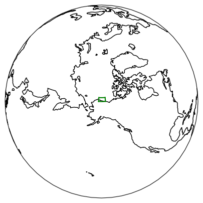
The grid for this model is located on the north slope of Alaska covering approximately 155-143\(^{\circ}\)W in longitude and 70-73\(^{\circ}\)N in latitude. The grid spacing will be 500 m and the grid will span 511 rows and 840 columns.

This grid is stored in a netCDF file which we can read in as follows:

# read in the model longitude and latitude
ds = nc4.Dataset('../../../data/alaskan_north_slope/NorthSlope_ncgrid.nc')
XC = ds.variables['XC'][:, :]
YC = ds.variables['YC'][:, :]
dXC = ds.variables['dxC'][:, :]
dYC = ds.variables['dyC'][:, :]
ds.close()

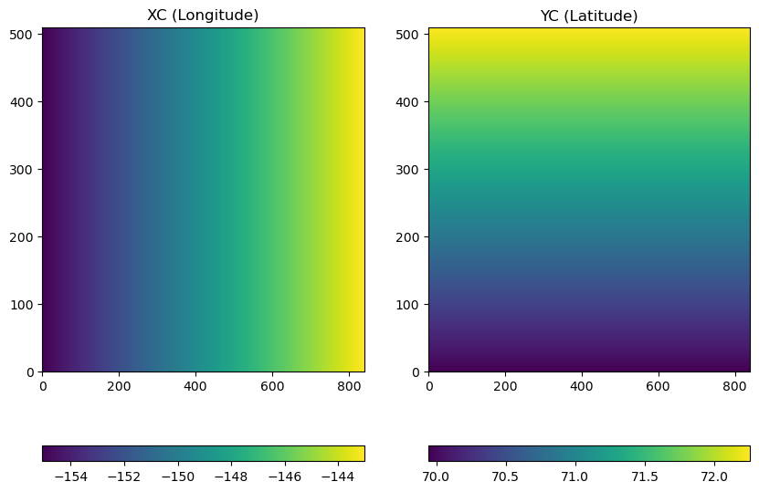
5.2.1.1. Visualizing the Grid

The grids above can be visualized as follows:

# make a plot of XC and YC
plt.figure(figsize=(10,7))

plt.subplot(1,2,1)
C = plt.pcolormesh(XC)
plt.colorbar(C, orientation = 'horizontal')
plt.title('XC (Longitude)')

plt.subplot(1,2,2)
C = plt.pcolormesh(YC)
plt.colorbar(C, orientation = 'horizontal')
plt.title('YC (Latitude)')

plt.show()

5.2.1.2. Visualizing the Grid on a Map with Cartopy

To get a sense of where the model is located on the globe, cartopy can be be used to plot the domain on the globe:

plt.figure(figsize=(5,5))
ax = plt.axes(projection=ccrs.Orthographic(-150,70))
ax.plot(XC[:,0], YC[:,0], 'g-', transform=ccrs.PlateCarree())
ax.plot(XC[:,-1], YC[:,-1], 'g-', transform=ccrs.PlateCarree())
ax.plot(XC[0,:], YC[0,:], 'g-', transform=ccrs.PlateCarree())
ax.plot(XC[-1,:], YC[-1,:], 'g-', transform=ccrs.PlateCarree())
ax.coastlines()
ax.set_global()
plt.show()

5.2.1.3. Visualizing the Grid Spacing

Here, we will visualize the grid spacing to ensure the dimensions match expectations:

# make a plot of XC and YC
plt.figure(figsize=(10,5))

plt.subplot(1,2,1)
C = plt.pcolormesh(dXC[:,1:])
plt.colorbar(C, orientation = 'horizontal')
plt.title('dXC')

plt.subplot(1,2,2)
C = plt.pcolormesh(dYC[1:,:])
plt.colorbar(C, orientation = 'horizontal')
plt.title('dYC')

plt.show()

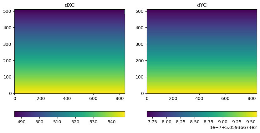
As we can see the grid has a resolution of about 500 m, although there is a north-south gradient in horizontal distances (in other words, points further north are closer together).