In this notebook, we will explore how to create the bathymetry of a model given its grid.

First, import packages to create and visualize the model grid and bathymetry here:

# import the packages for computation and visualization
import os
import numpy as np
from scipy.interpolate import griddata
import matplotlib.pyplot as plt
import netCDF4 as nc4

# import the bathymetry module from eccoseas
from eccoseas.downscale import bathymetry as edb

3.3.1. Generating the Bathymetry Grid

To generate the bathymetry for the model, first obtain a subset of the global GEBCO bathymetry grid from here: https://download.gebco.net/

For this model, requested a subset covering the grid ranging from 136-114\(^{\circ}\)W in longitude and 28-54\(^{\circ}\)N in latitude (i.e. one additional degree on all sides). Then, store the bathymetry as GEBCO_Bathymetry_California.nc into the ../../../data/ca directory to run the following cells.

3.3.1.1. Interpolating Bathymetry onto the Model Domain

Next, I use a standard interpolation function to interpolate the GEBCO Bathymetry onto the domain of my model.

# read in the bathymetry grid
file_path = '../../../data/ca/GEBCO_Bathymetry_California.nc'
ds = nc4.Dataset(file_path)
gebco_lon = ds.variables['lon'][:]
gebco_lat = ds.variables['lat'][:]
Gebco_bathy = ds.variables['elevation'][:]
ds.close()

# create a meshgrid of the lon and lat
Gebco_Lon, Gebco_Lat = np.meshgrid(gebco_lon, gebco_lat)

# recreate the model grid - see previous notebook on creating the model grid for details
delX = 1/12
delY = 1/16
xgOrigin = -135
ygOrigin = 29
n_rows = 360
n_cols = 240

xc = np.arange(xgOrigin+delX/2, xgOrigin+n_cols*delX, delX)
yc = np.arange(ygOrigin+delY/2, ygOrigin+n_rows*delY, delY)
XC, YC = np.meshgrid(xc, yc)
print('Double check shape:', np.shape(xc),np.shape(yc))

Double check shape: (240,) (360,)

# interpolate the gebco data onto the model grid
Model_bathy = griddata(np.column_stack([Gebco_Lon.ravel(),Gebco_Lat.ravel()]), Gebco_bathy.ravel(), (XC, YC), method='nearest')

# set points on land to 0
Model_bathy[Model_bathy>0] = 0

3.3.1.2. Visualizing the Bathymetry Grid

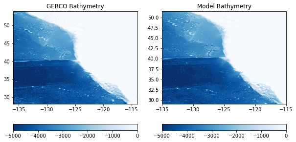
To ensure the interpolation went as planned, create a plot of the bathymetry and compare with the source data:

plt.figure(figsize=(10,5))

plt.subplot(1,2,1)
C = plt.pcolormesh(Gebco_Lon, Gebco_Lat, Gebco_bathy, vmin=-5000, vmax=0, cmap='Blues_r')
plt.colorbar(C, orientation = 'horizontal')
plt.title('GEBCO Bathymetry')

plt.subplot(1,2,2)
C = plt.pcolormesh(XC, YC, Model_bathy, vmin=-5000, vmax=0, cmap='Blues_r')
plt.colorbar(C, orientation = 'horizontal')
plt.title('Model Bathymetry')

plt.show()

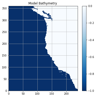
3.3.1.3. Checking for isolated regions

One potential problem that can be encountered in ocean models occurs with isolated regions. For example, if there is an artificial inland “lake” below sea level, such as Death Valley or the Salton Sea in California, the model will fill this with water and treat it as part of the ocean. Let’s see where these may be in our model:

plt.figure(figsize=(6,6))

C = plt.pcolormesh(Model_bathy, vmin=-1, vmax=0, cmap='Blues_r')
plt.colorbar(C)
plt.title('Model Bathymetry ')

plt.show()

As we can see, there are several isolated regions. In addition, there is an area of extreme detail in the area of British Columbia, Canada. This is sure to cause problems such as excess evaporation running the cell dry. To avoid these pitfalls, we will “fill” these regions before proceeding with the model.

The fill_unconnected_model_regions function from the bathymetry module is designed to do just that:

# fill the model by "spreading" outward from a known wet row and column (this may take a moment or two...)
Model_bathy = edb.fill_unconnected_model_regions(Model_bathy, central_wet_row=100, central_wet_col=100)

After filling, we can double check that the problem areas are now alleviated:

plt.figure(figsize=(6,6))

C = plt.pcolormesh(Model_bathy, vmin=-1, vmax=0, cmap='Blues_r')
plt.colorbar(C)
plt.grid()
plt.title('Model Bathymetry ')

plt.show()

3.3.1.4. Manually checking for problem areas

Another potential problem that can be encountered in ocean models occurs in regions where there is shallow bathymetry in enclosed bays. In these regions, there can be fast currents and strong dynamics. If this is your area of interest, then this is great! If not, it may cause problems in your domain. One option is to manually fill in these areas to avoid any potential issues.

In this example, the Juan de Fuca Strait between Canada and Washington State is filled artificially:

# fill in some areas around BC
Model_bathy_filled = np.copy(Model_bathy)
Model_bathy_filled[342:352, 85:105] = 0
Model_bathy_filled[280:340, 130:160] = 0
Model_bathy_filled[325:350, 115:130] = 0

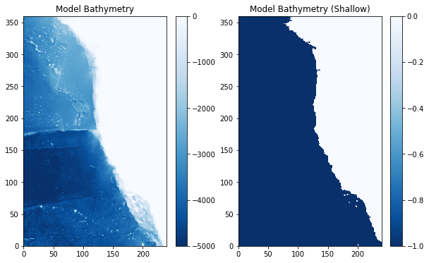
Again, plot the filled bathymetry to ensure it looks as expected:

plt.figure(figsize=(10,6))

plt.subplot(1,2,1)
C = plt.pcolormesh(Model_bathy_filled, vmin=-5000, vmax=0, cmap='Blues_r')
plt.colorbar(C)
plt.title('Model Bathymetry')

plt.subplot(1,2,2)
C = plt.pcolormesh(Model_bathy_filled, vmin=-1, vmax=0, cmap='Blues_r')
plt.colorbar(C)
plt.title('Model Bathymetry (Shallow)')

plt.show()

Once the bathymetry looks good, it can be output as a binary file to read in with MITgcm:

# make sure the input folder exists
if 'input' not in os.listdir('../../../configurations/california'):
    os.mkdir('../../../configurations/california/input')

# then, save the bathymetry in the input folder
output_file = '../../../configurations/california/input/CA_bathymetry.bin'
Model_bathy_filled.ravel('C').astype('>f4').tofile(output_file)